This use case is a customized time series forecasting version of making a CNN prediction model from the TensorFlow website.
The code is dived into multiple segments and expected output is posted to make sure there are no errors, making it easier to debug.
The complete tutorial is available on the TensorFlow website.
If you run the script below, you see an output of a DataFrame (table).
#### Initial Imports
import os
import datetime
import matplotlib as mpl
import matplotlib.pyplot as plt
import numpy as np
import pandas as pd
import seaborn as sns
import tensorflow as tf
### Optional for setting up plot sizes
mpl.rcParams['figure.figsize'] = (8, 6)
mpl.rcParams['axes.grid'] = False
### Get Data
zip_path = tf.keras.utils.get_file(
origin='https://storage.googleapis.com/tensorflow/tf-keras-datasets/jena_climate_2009_2016.csv.zip',
fname='jena_climate_2009_2016.csv.zip',
extract=True)
csv_path, _ = os.path.splitext(zip_path)
## Read Data into pandas data frame
df = pd.read_csv(csv_path)
# slice [start:stop:step], starting from index 5 take every 6th record.
df = df[5::6]
date_time = pd.to_datetime(df.pop('Date Time'), format='%d.%m.%Y %H:%M:%S')
print(df.head())
p (mbar) T (degC) Tpot (K) Tdew (degC) ... rho (g/m**3) wv (m/s) max. wv (m/s) wd (deg)
5 996.50 -8.05 265.38 -8.78 ... 1307.86 0.21 0.63 192.7
11 996.62 -8.88 264.54 -9.77 ... 1312.25 0.25 0.63 190.3
17 996.84 -8.81 264.59 -9.66 ... 1312.18 0.18 0.63 167.2
23 996.99 -9.05 264.34 -10.02 ... 1313.61 0.10 0.38 240.0
29 997.46 -9.63 263.72 -10.65 ... 1317.19 0.40 0.88 157.0
[5 rows x 14 columns]
Feature Engineering / Data Standardization
Now with the quick setup done, we can do some feature engineering / extraction and data manipulation which will help the model.
There are plenty of options when it comes to feature engineering and it is case-by-case basis, but for this example, it will be kept almost exactly the same as TensorFlow.
### Select as many or as little number of columns of variables
columns = ['p (mbar)','T (degC)','Tpot (K)','Tdew (degC)','rh (%)', 'VPmax (mbar)', 'VPact (mbar)', 'VPdef (mbar)', 'sh (g/kg)','H2OC (mmol/mol)','rho (g/m**3)','wv (m/s)', 'max. wv (m/s)', 'wd (deg)']
### A DataFrame containing the selected columns is named as "features" features = df[columns]
features.index = date_time
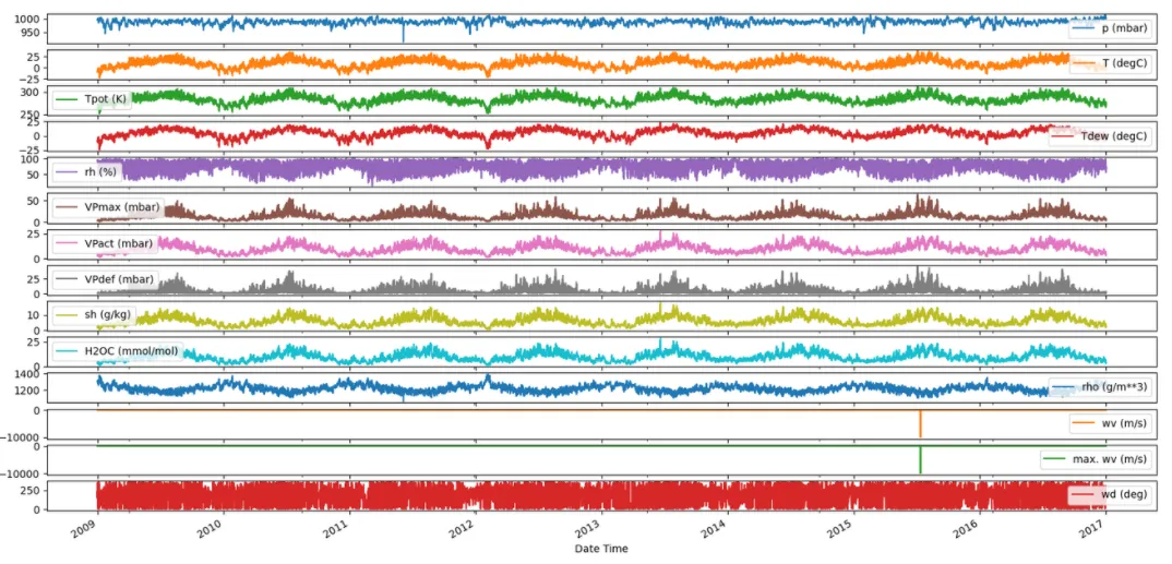
### Optional - If you want to see a plot of these features_ = features.plot(subplots=True)
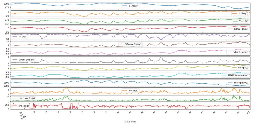
### Optional - smoother version of the plot by using only the first month of datafeatures = df[columns][:480]
features.index = date_time[:480]
_ = features.plot(subplots=True)
plt.show()
### To see the statistics of the selected data print(df.describe().transpose())
count mean std min 25% 50% 75% max
p (mbar) 70091.0 989.212842 8.358886 913.60 984.20 989.57 994.720 1015.29
T (degC) 70091.0 9.450482 8.423384 -22.76 3.35 9.41 15.480 37.28
Tpot (K) 70091.0 283.493086 8.504424 250.85 277.44 283.46 289.530 311.21
Tdew (degC) 70091.0 4.956471 6.730081 -24.80 0.24 5.21 10.080 23.06
rh (%) 70091.0 76.009788 16.474920 13.88 65.21 79.30 89.400 100.00
VPmax (mbar) 70091.0 13.576576 7.739883 0.97 7.77 11.82 17.610 63.77
VPact (mbar) 70091.0 9.533968 4.183658 0.81 6.22 8.86 12.360 28.25
VPdef (mbar) 70091.0 4.042536 4.898549 0.00 0.87 2.19 5.300 46.01
sh (g/kg) 70091.0 6.022560 2.655812 0.51 3.92 5.59 7.800 18.07
H2OC (mmol/mol) 70091.0 9.640437 4.234862 0.81 6.29 8.96 12.490 28.74
rho (g/m**3) 70091.0 1216.061232 39.974263 1059.45 1187.47 1213.80 1242.765 1393.54
wv (m/s) 70091.0 1.702567 65.447512 -9999.00 0.99 1.76 2.860 14.01
max. wv (m/s) 70091.0 2.963041 75.597657 -9999.00 1.76 2.98 4.740 23.50
wd (deg) 70091.0 174.789095 86.619431 0.00 125.30 198.10 234.000 360.00
Plot of initial part of data set
Plot of initial part of data set
Most of this section is highly dependent on the kind of data being used. This data is of the weather, and various parameters are used to predict the temperature. So most of this cleanup is specific to these kinds of datasets, and maybe completely irrelevant to other kinds of datasets.
As the minimum value of wind velocity (wv m/s) and max. wv m/s is -9999, it seems incorrect, as we already have wind direction, let's correct this minimum.
wv = df['wv (m/s)']
bad_wv = wv == -9999.0
wv[bad_wv] = 0.0
max_wv = df['max. wv (m/s)']
bad_max_wv = max_wv == -9999.0
max_wv[bad_max_wv] = 0.0
### check if original data frame is edited correctly print(df['wv (m/s)'].min())
### Expected value 0.0
Note: This may not apply to all kinds of datasets.
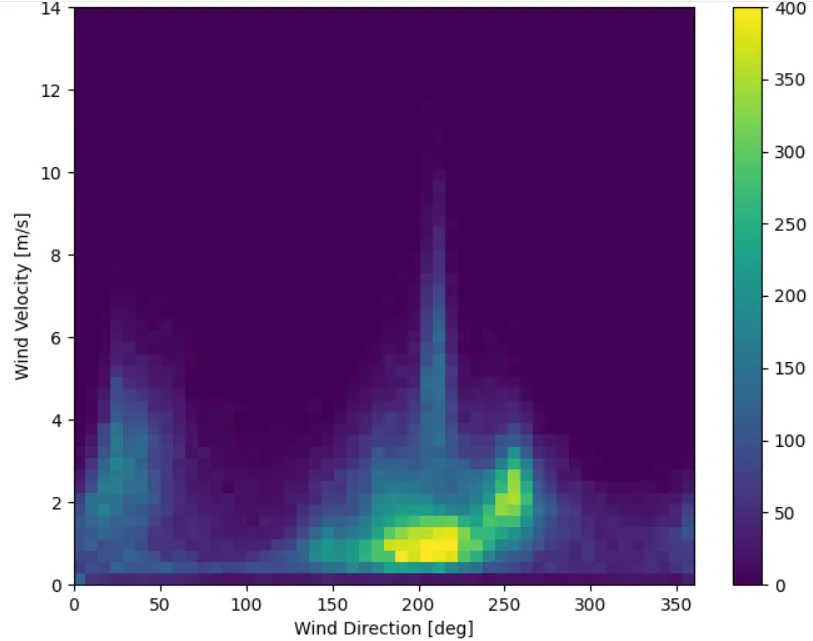
To see why we need to change the wind variables, lets plot them first.
plt.figure()
plt.hist2d(df['wd (deg)'], df['wv (m/s)'], bins=(50, 50), vmax=400)
plt.colorbar()
plt.xlabel('Wind Direction [deg]')
plt.ylabel('Wind Velocity [m/s]')
### If you forgot to add this earlier
### plt.show()
Not to get into too many details, but ideally 0 degrees and 360 degrees should be next to each other, which they aren't - and it should not be a sharp change at 0 degree mark. Also, direction of the wind does not matter if its velocity is 0 (no wind).
So let's make some changes to the DataFrame and make wind velocity a vector, rather than scalar with degrees.
### Remove these columns from the data frame and replace them as vectors
wv = df.pop('wv (m/s)')
max_wv = df.pop('max. wv (m/s)')
### Convert to radians
wd_rad = df.pop('wd (deg)')*np.pi / 180
### Calculate the wind x and y components df['Wx'] = wvnp.cos(wd_rad)
df['Wy'] = wvnp.sin(wd_rad)
### Calculate the max wind x and y components df['max Wx'] = max_wvnp.cos(wd_rad)
df['max Wy'] = max_wvnp.sin(wd_rad)
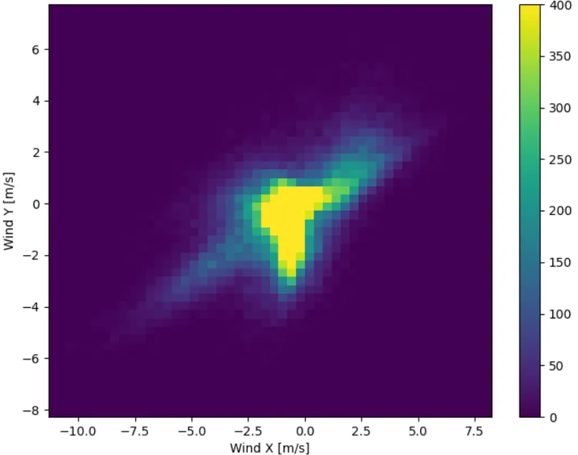
### check the histogram again, with better representation of wind variables plt.figure()
plt.hist2d(df['Wx'], df['Wy'], bins=(50, 50), vmax=400)
plt.colorbar()
plt.xlabel('Wind X [m/s]')
plt.ylabel('Wind Y [m/s]')
ax = plt.gca()
ax.axis('tight')
### plt.show()
The model interprets this kind of wind variables better than it does with velocity and direction.
### Optional - Check your data frame again to see what modifications have been made so far
print(df.head())
print(df.describe().transpose())
p (mbar) T (degC) Tpot (K) Tdew (degC) ... Wx Wy max Wx max Wy
5 996.50 -8.05 265.38 -8.78 ... -0.204862 -0.046168 -0.614587 -0.138503
11 996.62 -8.88 264.54 -9.77 ... -0.245971 -0.044701 -0.619848 -0.112645
17 996.84 -8.81 264.59 -9.66 ... -0.175527 0.039879 -0.614344 0.139576
23 996.99 -9.05 264.34 -10.02 ... -0.050000 -0.086603 -0.190000 -0.329090
29 997.46 -9.63 263.72 -10.65 ... -0.368202 0.156292 -0.810044 0.343843
[5 rows x 15 columns]
count mean std ... 50% 75% max
p (mbar) 70091.0 989.212842 8.358886 ... 989.570000 994.720000 1015.290000
T (degC) 70091.0 9.450482 8.423384 ... 9.410000 15.480000 37.280000
Tpot (K) 70091.0 283.493086 8.504424 ... 283.460000 289.530000 311.210000
Tdew (degC) 70091.0 4.956471 6.730081 ... 5.210000 10.080000 23.060000
rh (%) 70091.0 76.009788 16.474920 ... 79.300000 89.400000 100.000000
VPmax (mbar) 70091.0 13.576576 7.739883 ... 11.820000 17.610000 63.770000
VPact (mbar) 70091.0 9.533968 4.183658 ... 8.860000 12.360000 28.250000
VPdef (mbar) 70091.0 4.042536 4.898549 ... 2.190000 5.300000 46.010000
sh (g/kg) 70091.0 6.022560 2.655812 ... 5.590000 7.800000 18.070000
H2OC (mmol/mol) 70091.0 9.640437 4.234862 ... 8.960000 12.490000 28.740000
rho (g/m**3) 70091.0 1216.061232 39.974263 ... 1213.800000 1242.765000 1393.540000
Wx 70091.0 -0.627813 1.987440 ... -0.633142 0.299975 8.244699
Wy 70091.0 -0.407068 1.552621 ... -0.293467 0.450077 7.733831
max Wx 70091.0 -1.018681 3.095279 ... -1.117029 0.627619 11.913133
max Wy 70091.0 -0.733589 2.611890 ... -0.527021 0.822895 14.302308
We took our desired number of features/columns from the original data set
Modified the data such that there is no -9999 as the minimum value in the wind velocity
Changed wind variables from wind velocity + wind direction (degrees) into -> wind velocity vector in x & y components
Timestamp, date-time in string, time in seconds is not really that useful for the model, so we can make features instead.
We can convert date-time to seconds, and then to sin & cos of years and days. This will help simplify input to the model and make it more useful to identify periodicity in the data.
### Convert timestamp in data to seconds
timestamp_s = date_time.map(datetime.datetime.timestamp)
day = 246060
year = (365.2425)*day
### Make useful features out of this for the data frame
df['Day sin'] = np.sin(timestamp_s * (2 * np.pi / day))
df['Day cos'] = np.cos(timestamp_s * (2 * np.pi / day))
df['Year sin'] = np.sin(timestamp_s * (2 * np.pi / year))
df['Year cos'] = np.cos(timestamp_s * (2 * np.pi / year))
### To see how this is useful for the model, try visualizing it in terms of frequency
### This part is only if you want to know how the above features will be helpful to the model
### no other changes will be made with the following
# fft = tf.signal.rfft(df['T (degC)'])
# f_per_dataset = np.arange(0, len(fft))
# n_samples_h = len(df['T (degC)'])
# hours_per_year = 24*365.2524
# years_per_dataset = n_samples_h/(hours_per_year)
# f_per_year = f_per_dataset/years_per_dataset
# plt.figure()
# plt.step(f_per_year, np.abs(fft))
# plt.xscale('log')
# plt.ylim(0, 400000)
# plt.xlim([0.1, max(plt.xlim())])
# plt.xticks([1, 365.2524], labels=['1/Year', '1/day'])
# _ = plt.xlabel('Frequency (log scale)')
Preparing Data for the Model
All the necessary cleanups and some modifications to the data are done, now let's prepare the data for the model.
Split the data into training, validation and testing with ratios training-70% , validation-20%, testing-10%.
column_indices = {name: i for i, name in enumerate(df.columns)}
n = len(df)
train_df = df[0:int(n*0.7)]
val_df = df[int(n*0.7):int(n*0.9)]
test_df = df[int(n*0.9):]
num_features = df.shape[1]
Use the simple mean to normalize the data.
train_mean = train_df.mean()
train_std = train_df.std()
train_df = (train_df - train_mean) / train_std
val_df = (val_df - train_mean) / train_std
test_df = (test_df - train_mean) / train_std
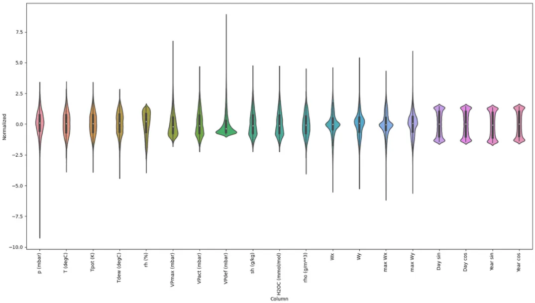
df_std = (df - train_mean) / train_std
df_std = df_std.melt(var_name='Column', value_name='Normalized')
Quick View of How the Data Looks
plt.figure(figsize=(12, 6))
ax = sns.violinplot(x='Column', y='Normalized', data=df_std)
_ = ax.set_xticklabels(df.keys(), rotation=90)
### plt.show()
Functions for Making a Moving Window Generator and Making Plots
This process is a methodology. You can also use other methods. See the TensorFlow website for more information.
### Indexes and Offsets
class WindowGenerator():
def init(self, input_width, label_width, shift,
train_df=train_df, val_df=val_df, test_df=test_df,
label_columns=None):
# Store the raw data.
self.train_df = train_df
self.val_df = val_df
self.test_df = test_df
# Work out the label column indices.
self.label_columns = label_columns
if label_columns is not None:
self.label_columns_indices = {name: i for i, name in
enumerate(label_columns)}
self.column_indices = {name: i for i, name in
enumerate(train_df.columns)}
# Work out the window parameters.
self.input_width = input_width
self.label_width = label_width
self.shift = shift
self.total_window_size = input_width + shift
self.input_slice = slice(0, input_width)
self.input_indices = np.arange(self.total_window_size)[self.input_slice]
self.label_start = self.total_window_size - self.label_width
self.labels_slice = slice(self.label_start, None)
self.label_indices = np.arange(self.total_window_size)[self.labels_slice]
def repr(self):
return '\n'.join([
f'Total window size: {self.total_window_size}',
f'Input indices: {self.input_indices}',
f'Label indices: {self.label_indices}',
f'Label column name(s): {self.label_columns}'])
### Split Window
def split_window(self, features):
inputs = features[:, self.input_slice, :]
labels = features[:, self.labels_slice, :]
if self.label_columns is not None:
labels = tf.stack(
[labels[:, :, self.column_indices[name]] for name in self.label_columns],
axis=-1)
# Slicing doesn't preserve static shape information, so set the shapes
# manually. This way the tf.data.Datasets are easier to inspect.
inputs.set_shape([None, self.input_width, None])
labels.set_shape([None, self.label_width, None])
return inputs, labels
WindowGenerator.split_window = split_window
### Plotting
def plot(self, model=None, plot_col='T (degC)', max_subplots=3):
inputs, labels = self.example
plt.figure(figsize=(12, 8))
plot_col_index = self.column_indices[plot_col]
max_n = min(max_subplots, len(inputs))
for n in range(max_n):
plt.subplot(3, 1, n+1)
plt.ylabel(f'{plot_col} [normed]')
plt.plot(self.input_indices, inputs[n, :, plot_col_index],
label='Inputs', marker='.', zorder=-10)
if self.label_columns:
label_col_index = self.label_columns_indices.get(plot_col, None)
else:
label_col_index = plot_col_index
if label_col_index is None:
continue
plt.scatter(self.label_indices, labels[n, :, label_col_index],
edgecolors='k', label='Labels', c='#2ca02c', s=64)
if model is not None:
predictions = model(inputs)
plt.scatter(self.label_indices, predictions[n, :, label_col_index],
marker='X', edgecolors='k', label='Predictions',
c='#ff7f0e', s=64)
if n == 0:
plt.legend()
plt.xlabel('Time [h]')
WindowGenerator.plot = plot
### Creating TF datasets
def make_dataset(self, data):
data = np.array(data, dtype=np.float32)
ds = tf.keras.preprocessing.timeseries_dataset_from_array(
data=data,
targets=None,
sequence_length=self.total_window_size,
sequence_stride=1,
shuffle=True,
batch_size=32,)
ds = ds.map(self.split_window)
return ds
WindowGenerator.make_dataset = make_dataset
### Add properties for window generators such as train, validation, test
@property
def train(self):
return self.make_dataset(self.train_df)
@property
def val(self):
return self.make_dataset(self.val_df)
@property
def test(self):
return self.make_dataset(self.test_df)
@property
def example(self):
"""Get and cache an example batch of inputs, labels for plotting."""
result = getattr(self, '_example', None)
if result is None:
# No example batch was found, so get one from the .train dataset
result = next(iter(self.train))
# And cache it for next time
self._example = result
return result
WindowGenerator.train = train
WindowGenerator.val = val
WindowGenerator.test = test
WindowGenerator.example = example
Extremely Simplistic Model
To truly understand what is going on, let's define a very simple model, which uses the variables that are currently in place, and makes a prediction for the next hour.
### OPTIONAL
### very simple model - predicts 1 timestamp (1hr) in the future
### generate window for the simple model
single_step_window = WindowGenerator(
input_width=1, label_width=1, shift=1,
label_columns=['T (degC)'])
### 1 timetamp is inputed, and prediction is made 1 hr in the future for the field "T (degC)"
print(single_step_window)
### shows you what the batch size is, how many timstamps consumed by input/ predicted by output and the number of features used/number of labels in the output (in out case only 1 label in output - T degC )
for example_inputs, example_labels in single_step_window.train.take(1):
print(f'Inputs shape (batch, time, features): {example_inputs.shape}')
print(f'Labels shape (batch, time, features): {example_labels.shape}')
### Create extremely basic model to be fed by the above window
class Baseline(tf.keras.Model):
def init(self, label_index=None):
super().init()
self.label_index = label_index
def call(self, inputs):
if self.label_index is None:
return inputs
result = inputs[:, :, self.label_index]
return result[:, :, tf.newaxis]
baseline = Baseline(label_index=column_indices['T (degC)'])
baseline.compile(loss=tf.losses.MeanSquaredError(),
metrics=[tf.metrics.MeanAbsoluteError()])
val_performance = {}
performance = {}
val_performance['Baseline'] = baseline.evaluate(single_step_window.val)
Total window size: 2
Input indices: [0]
Label indices: [1]
Label column name(s): ['T (degC)']
Inputs shape (batch, time, features): (32, 1, 19)
Labels shape (batch, time, features): (32, 1, 1)
439/439 [==============================] - 2s 5ms/step - loss: 0.0128 - mean_absolute_error: 0.0785
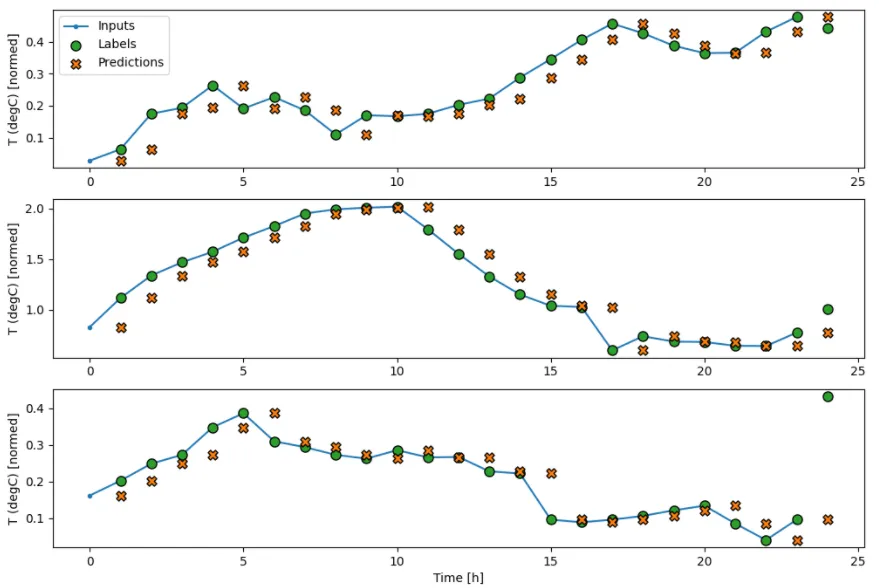
To make the model more interesting, repeat this window for 24 hrs instead just 1 hr.
### OPTIONAL
wide_window = WindowGenerator(
input_width=24, label_width=24, shift=1,
label_columns=['T (degC)'])
print(wide_window)
print('Input shape:', single_step_window.example[0].shape)
print('Output shape:', baseline(single_step_window.example[0]).shape)
wide_window.plot(baseline)
### plt.show()
Total window size: 25
Input indices: [ 0 1 2 3 4 5 6 7 8 9 10 11 12 13 14 15 16 17 18 19 20 21 22 23]
Label indices: [ 1 2 3 4 5 6 7 8 9 10 11 12 13 14 15 16 17 18 19 20 21 22 23 24]
Label column name(s): ['T (degC)']
Input shape: (32, 1, 19)
Output shape: (32, 1, 1)
Three Batches of the Basic Model
Three batches of the basic model
MAX_EPOCHS = 20
### make a function to be able to quickly compile and fit model
def compile_and_fit(model, window, patience=2):
early_stopping = tf.keras.callbacks.EarlyStopping(monitor='val_loss',
patience=patience,
mode='min')
model.compile(loss=tf.losses.MeanSquaredError(),
optimizer=tf.optimizers.Adam(),
metrics=[tf.metrics.MeanAbsoluteError()])
history = model.fit(window.train, epochs=MAX_EPOCHS,
validation_data=window.val,
callbacks=[early_stopping])
return history
### Use this much data
CONV_WIDTH = 48
### how many values to predict
LABEL_WIDTH = 1
### for plotting purposes
INPUT_WIDTH = LABEL_WIDTH + (CONV_WIDTH - 1)
### how many timesteps in future is the predicted value
SHIFT = 12
conv_window = WindowGenerator(
input_width = INPUT_WIDTH,
label_width = LABEL_WIDTH,
shift = SHIFT,
label_columns = ['T (degC)'])
print(conv_window)
### CNN model
conv_model = tf.keras.Sequential([
tf.keras.layers.Conv1D(filters=32,
kernel_size=(CONV_WIDTH,),
activation='relu'),
tf.keras.layers.Dense(units=32, activation='relu'),
tf.keras.layers.Dense(units=1, name='predict'),
])
print("Conv model on conv_window")
print('Input shape:', conv_window.example[0].shape)
print('Output shape:', conv_model(conv_window.example[0]).shape)
history = compile_and_fit(conv_model, conv_window)
val_performance['Conv'] = conv_model.evaluate(conv_window.val)
performance['Conv'] = conv_model.evaluate(conv_window.test, verbose=0)
conv_model.summary()
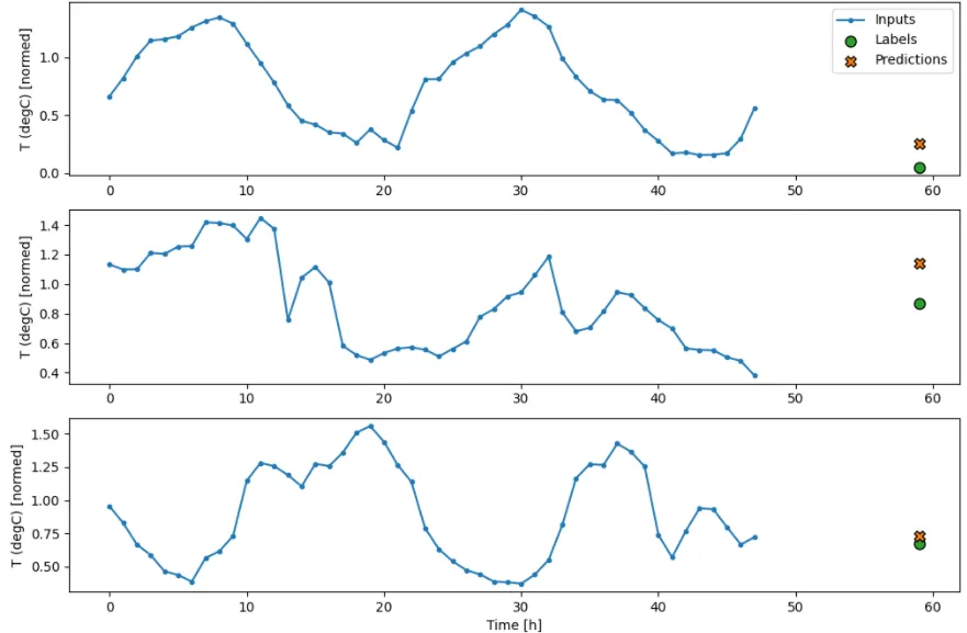
conv_window.plot(conv_model)
Total window size: 60
Input indices: [ 0 1 2 3 4 5 6 7 8 9 10 11 12 13 14 15 16 17 18 19 20 21 22 23
24 25 26 27 28 29 30 31 32 33 34 35 36 37 38 39 40 41 42 43 44 45 46 47]
Label indices: [59]
Label column name(s): ['T (degC)']
Conv model on conv_window
Input shape: (32, 48, 19)
Output shape: (32, 1, 1)
Epoch 1/20
1532/1532 [==============================] - 12s 8ms/step - loss: 0.1032 - mean_absolute_error: 0.2499 - val_loss: 0.1030 - val_mean_absolute_error: 0.2499
Epoch 2/20
1532/1532 [==============================] - 11s 7ms/step - loss: 0.0859 - mean_absolute_error: 0.2289 - val_loss: 0.0965 - val_mean_absolute_error: 0.2427
Epoch 3/20
1532/1532 [==============================] - 12s 8ms/step - loss: 0.0802 - mean_absolute_error: 0.2204 - val_loss: 0.1005 - val_mean_absolute_error: 0.2490
Epoch 4/20
1532/1532 [==============================] - 11s 7ms/step - loss: 0.0764 - mean_absolute_error: 0.2152 - val_loss: 0.1084 - val_mean_absolute_error: 0.2593
437/437 [==============================] - 2s 5ms/step - loss: 0.1084 - mean_absolute_error: 0.2593
Model: "sequential"
Layer (type) Output Shape Param #
conv1d (Conv1D) (None, 1, 32) 29216
dense (Dense) (None, 1, 32) 1056
predict (Dense) (None, 1, 1) 33
Total params: 30,305
Trainable params: 30,305
Non-trainable params: 0
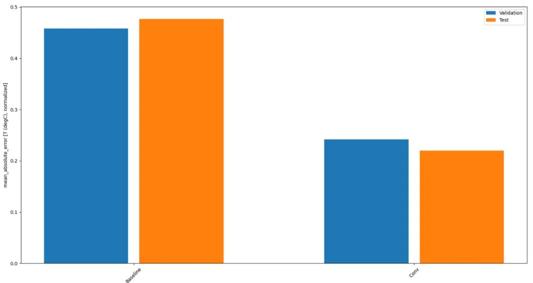
### Compare performances
x = np.arange(len(performance))
width = 0.3
metric_name = 'mean_absolute_error'
metric_index = conv_model.metrics_names.index('mean_absolute_error')
val_mae = [v[metric_index] for v in val_performance.values()]
test_mae = [v[metric_index] for v in performance.values()]
plt.figure()
plt.ylabel('mean_absolute_error [T (degC), normalized]')
plt.bar(x - 0.17, val_mae, width, label='Validation')
plt.bar(x + 0.17, test_mae, width, label='Test')
plt.xticks(ticks=x, labels=performance.keys(),
rotation=45)
_ = plt.legend()
plt.show()
Saving a model in Keras is simple.
### Replace enter the path (in string) where you want to save the model, and then the name of the model with a /
conv_model.save("{PATH_TO_SAVE_MODEL}/{NAME_OF_SAVED_MODEL}")
### How to load a model
# model = tf.keras.models.load_model("{PATH_TO_SAVE_MODEL}/{NAME_OF_SAVED_MODEL}")
# print("loaded")
# model.summary()
### How to check all the input tensors and output tensor names
# print(os.system("saved_model_cli show --dir {PATH_TO_SAVE_MODEL}/{NAME_OF_SAVED_MODEL} --all"))
MetaGraphDef with tag-set: 'serve' contains the following SignatureDefs:
signature_def['__saved_model_init_op']:
The given SavedModel SignatureDef contains the following input(s):
The given SavedModel SignatureDef contains the following output(s):
outputs['__saved_model_init_op'] tensor_info:
dtype: DT_INVALID
shape: unknown_rank
name: NoOp
Method name is:
signature_def['serving_default']:
The given SavedModel SignatureDef contains the following input(s):
inputs['conv1d_input'] tensor_info:
dtype: DT_FLOAT
shape: (-1, 48, 19)
name: serving_default_conv1d_input:0
The given SavedModel SignatureDef contains the following output(s):
outputs['predict'] tensor_info:
dtype: DT_FLOAT
shape: (-1, 1, 1)
name: StatefulPartitionedCall:0
Method name is: tensorflow/serving/predict
Defined Functions:
Function Name: 'call'
Option #1
Callable with:
Argument #1
inputs: TensorSpec(shape=(None, 48, 19), dtype=tf.float32, name='inputs')
Argument #2
DType: bool
Value: False
Argument #3
DType: NoneType
Value: None
Option #2
Callable with:
Argument #1
conv1d_input: TensorSpec(shape=(None, 48, 19), dtype=tf.float32, name='conv1d_input')
Argument #2
DType: bool
Value: False
Argument #3
DType: NoneType
Value: None
Option #3
Callable with:
Argument #1
inputs: TensorSpec(shape=(None, 48, 19), dtype=tf.float32, name='inputs')
Argument #2
DType: bool
Value: True
Argument #3
DType: NoneType
Value: None
Option #4
Callable with:
Argument #1
conv1d_input: TensorSpec(shape=(None, 48, 19), dtype=tf.float32, name='conv1d_input')
Argument #2
DType: bool
Value: True
Argument #3
DType: NoneType
Value: None
Function Name: '_default_save_signature'
Option #1
Callable with:
Argument #1
conv1d_input: TensorSpec(shape=(None, 48, 19), dtype=tf.float32, name='conv1d_input')
Function Name: 'call_and_return_all_conditional_losses'
Option #1
Callable with:
Argument #1
conv1d_input: TensorSpec(shape=(None, 48, 19), dtype=tf.float32, name='conv1d_input')
Argument #2
DType: bool
Value: True
Argument #3
DType: NoneType
Value: None
Option #2
Callable with:
Argument #1
conv1d_input: TensorSpec(shape=(None, 48, 19), dtype=tf.float32, name='conv1d_input')
Argument #2
DType: bool
Value: False
Argument #3
DType: NoneType
Value: None
Option #3
Callable with:
Argument #1
inputs: TensorSpec(shape=(None, 48, 19), dtype=tf.float32, name='inputs')
Argument #2
DType: bool
Value: True
Argument #3
DType: NoneType
Value: None
Option #4
Callable with:
Argument #1
inputs: TensorSpec(shape=(None, 48, 19), dtype=tf.float32, name='inputs')
Argument #2
DType: bool
Value: False
Argument #3
DType: NoneType
Value: None